Troubleshooting Abaqus/Explicit analyses that use contact pairs

This blog explains the different errors encountered while using Abaqus/Explicit and the ways to debug and troubleshoot them.

    1. Tracking Difficulties

Reason: By default, Abaqus/Explicit uses a fast, local tracking algorithm to track the penetration of a slave node into the master surface; at a frequency of every 100 increments (the user can change this default), Abaqus/Explicit performs a global search. If penetration by a slave node goes undetected for a period of time (in between the global searches), the code may allow the penetration to go unresolved and a large correction (or force) may be required to overcome the penetration when it is finally detected. A high velocity is imparted to the nodes that had penetrated the contact surfaces but were not detected as over-penetrated; this high rate of deformation causes problems such as severe element distortion.

Debugging: Create a history plot of global energy quantities ALLIE and ALLKE for every time increment prior to termination. If a contact correction is the reason for termination, there will be a large spike in ALLKE just prior to the termination point.

In addition, create vector plots of A and CFORCE from the state just prior to termination. Look for evidence of contact force values and accelerations (and the corresponding locations) that are much higher than elsewhere in the model, particularly on contact surfaces and in the region of the node or element number indicated in the error message.

If necessary, rerun or restart the analysis to get this information. If the penetration goes undetected during the analysis, no diagnostic messages will be printed. However, this problem can be seen by looking at the deformed shape of the model and checking that the contact pressures and opening make sense.

Caution: In the event of a restart analysis, the problem might not reproduce itself due to step initialization and the fact that the initial time increment will not replicate the one used in the original analysis (at the start of every step, an element-by-element time estimator is used; later, a global time estimator is used). If you are running a multi-step analysis and several steps complete prior to termination, it is better to restart from the beginning of the last completed step.

Remedy: Increase the frequency of the global contact tracking

    • Abaqus/CAE: Interaction Module: Interaction → Contact Controls → Create… → Global Search Frequency
    • Keyword: *CONTACT CONTROLS, CPSET=contact_pair_set_name, GLOBALTRKINC=n and/or use the more conservative local tracking algorithm
    • Abaqus/CAE: Interaction Module: Interaction → Contact Controls → Create… → unselect Fast local tracking
    • Keyword: *CONTACT CONTROLS, CPSET=contact_pair_set_name, FASTLOCALTRK=NO
    1. Hourglassing

Reason: Abaqus/Explicit generally offers first-order reduced-integration elements, which may be susceptible to hourglassing. When mesh refinement is inadequate, hourglassing may cause nonphysical deformation modes that, when coupled with contact constraints, can lead to severe contact penetrations. This is particularly true when contact occurs at a single node.

Debugging: Plot the global energy histories ALLIE and ALLAE for all increments up to termination. If ALLAE is a significant fraction of ALLIE, hourglassing has occurred. In addition, inspect the deformation pattern of the mesh at times prior to failure. If a regular pattern of element distortion is clearly visible in the deformed mesh (you may have to increase the magnification factor to see it), hourglassing is probably occurring.

Remedy: The enhanced hourglass control method, which is based on the enhanced assumed strain method, may help. Use:

      • Abaqus/CAE: Mesh module: Mesh → Element Type… → Hourglass control: Enhanced
      • Keyword: *SECTION CONTROLS, NAME=name, HOURGLASS=ENHANCED

If you have decided not to use the enhanced hourglass control approach, refine the mesh and try to distribute the contact over several nodes (for example, change sharp corners to round corners). Increasing the hourglass stiffness is usually not the best solution. If mesh refinement does not cure the hourglassing, try using a different type of hourglass control.

If you need to increase the hourglass stiffness, use:

    • Abaqus/CAE: Mesh module: Mesh → Element Type… → Hourglass control: type_of_hourglass_control
    • Keyword: *SECTION CONTROLS, NAME=name, HOURGLASS=type_of_hourglass_control where type_of_hourglass_controlis:
      • RELAX STIFFNESS for the default integral viscoelastic approach
      • STIFFNESS for the Kelvin viscoelastic stiffness approach
      • VISCOUS for the Kelvin viscoelastic viscous approach
      • COMBINED, WEIGHT FACTOR= for the stiffness and viscous Kelvin viscoelastic approach
    1. Material instability

Reason: Material instability may occur near a contact interface because contact may be the first type of loading on a structure. Since contact is frequently a sudden load (such as in an impact), the loading may be severe enough to cause the material to go unstable.

Debugging: Usually this problem is characterized by a large acceleration without a corresponding large reaction force at a contact node (the acceleration is due to the element’s internal force rather than an external force).

Remedy: Check the material definition to ensure stability requirements are satisfied (in particular for hyper elastic materials). If the material stability requirements are met, try applying the contact gradually to reduce its severity. Use velocity boundary conditions, or use the smooth-step amplitude definition.

    1. Initial overclosures

Reason: Abaqus/Explicit does not permit any initial overclosures. The nodes on the contacting surfaces are adjusted to remove the initial overclosure. Corrections at the beginning of an analysis do not induce strains; later adjustments cause strains. Thus, if the initial overclosure is too large in steps other than the first, the corresponding contact correction may be too large and cause significant deformation in the elements.

With balanced master-slave contact or when nodes are slaves to more than one master surface (i.e., pinched contact), it is possible to have unresolved initial overclosures. These will result in large initial accelerations, which can lead to significant mesh distortion. The unresolved overclosures are reported to the status (.sta) file.

Adjacent slave nodes (i.e., those connected by a facet) that initially lie on either side of a double-sided surface will be corrected so that each slave node is moved to the nearest free surface (thus, the slave nodes will be moved to opposite sides of the master surface).

Warnings for such a case are issued when the slave nodes are defined as part of a surface but not when they are defined through node-based surfaces (i.e., contact node sets). This will lead to contact difficulties if not corrected.

Debugging: Check your model for evidence of initial overclosures. In particular, remember to consider the thickness of a shell when positioning bodies relative to one another. If introducing a new contact pair in a later step (for example, adding a new rigid punch and die), take into account any deformations that may have occurred up to that point when positioning the new features.

In addition, check for incorrect surface normals. For single-sided contact the surface normal must be consistent and point toward the opposing surface.

To understand what is happening, try to simplify the model to include only the region near the large accelerations. Adjusting the weighting of the contact pair (or pairs) often helps.

Remedy: Reposition surfaces to remove the initial overclosures. Reverse surface normal definitions if necessary. If surfaces are being pinched, make the pinched surfaces master surfaces if possible.

    1. Overconstraining the model with MPCs and equations

Reason: Overconstraining nodes with MPCs or equations and contact conditions can generate conflicting constraints when using kinematic contact. In some cases this can lead to large distortions and contact corrections.

Debugging: Remove the constraints one at a time to isolate the culprit.

Remedy: Redefine or remove the constraints. Switching to penalty contact will tend to alleviate the problem as well.

    1. Highly warped surfaces

Reason: It is difficult to calculate the correct contact conditions when surfaces are, or become, highly warped. Warping is monitored throughout the analysis at regular intervals, and warnings are issued when warping exceeds a threshold value (the default is 20 degrees). If this happens, Abaqus/Explicit switches to a more accurate algorithm to determine the nearest point on the master surface for a slave node.

Debugging: Significant warping is sometimes an indication of problems in the solution, so Abaqus/Explicit issues a warning message in the status (.sta) file when a threshold value of warping is exceeded (the default is 20 degrees between surface normals of adjacent elements). This message is more of an indicator of solution problems if the underlying elements of the surface are solid elements — in this case, warping is frequently a sign of hourglassing. This is a less common cause for shells and membranes. Frequently, the problems caused by highly warped surfaces in contact will trigger the “excessive wave speed” error.

Remedy: Refine the underlying surface mesh if possible, and make sure that the surface is modelled as smoothly as possible.

    1. Inadequate surface definitions

Reason: Penetrations may occur because a surface is improperly or inadequately defined. For example, if large deformations are expected, the underlying surface must extend far enough to prevent a slave node from sliding around the end of the master surface. If this happens (the slave node gets behind the master surface), the slave node will be forced immediately to the master surface (to satisfy the contact constraint). This will impart very large forces and velocities to the slave node, probably causing severe element distortion.

If two-sided contact is possible (in a shell model), the contact surface must be defined properly as a double-sided contact surface.

If the contact is pure master-slave, the master surface nodes can penetrate the slave surface.

Debugging: Check the surface definitions:

      • Do they need to be extended so that slave nodes do not slide behind master surfaces?
      • Is two-sided contact possible?
      • Does the contact pair weighting need to be adjusted?
      • Are the masses of the master and slave surfaces very different?
      • Is the edge of a surface a symmetry boundary condition?

Remedy: Make sure that the surfaces extend far enough so that nodal penetrations are prevented. When modelling contacts with shell elements, use two-sided contact.

If the edge of a surface is a symmetry boundary, remember to put the symmetry boundary condition on both the slave and master surfaces.

    1. Self-contact with thick shells

Reason: The shell thickness is considered in contact calculations. Extremely large thicknesses (greater than the spacing between nodes) will cause nodes to appear to be penetrating nearby facets even in a flat self-contact surface (a node “penetrates” the outer boundary of its neighbour even when it is impossible for it to do so physically).

Debugging: Compare the shell thickness against a typical element dimension (edge or diagonal length).

Remedy: Use the SCALE THICK and/or MAXRATIO parameters on the *SURFACE option to scale down the thickness used in the contact calculations on the elements forming a surface. Make sure the contact thickness is still significant relative to the facet size.

    1. Contact with thick shells

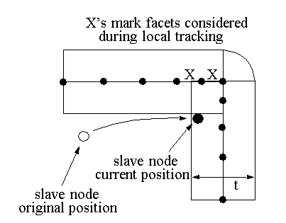
 Reason: There is a chance of encountering tracking problems at corners (for example, only facets on one side of a corner might be considered during local tracking, but when the global tracking is done, a slave node might be detected as being over-penetrated by facets on the other edge of the corner).
Troubleshooting Abaqus-Explicit analyses that use contact pairs-1

The slave node in the current position will be forced back onto the contact surface, resulting in large contact forces and velocities.

Debugging: Compare the shell thickness against a typical element dimension (edge or diagonal length).

Remedy: Either use the NO THICK parameter on the *SURFACE option to completely ignore the element thickness when performing contact calculations. More frequent global tracking of the contact may also help.

    1. Poor surface definition with shell offsets

Reason: At acute corners shell offsets may result in a poorly defined contact surface (tangled midsurface). Since tracking is based on the shell midsurface, you can encounter tracking problems with a tangled surface.

Debugging: Compare the shell thickness against a typical element dimension (edge or diagonal length).

Remedy: Use the NO OFFSET parameter on the *SURFACE option to ignore the shell section offset when performing contact calculations.

    1. Excessive loading rates/excessive mass scaling

Reason: By default, loads are applied instantaneously. This type of loading imparts large kinetic energy to nodes, possibly causing excessive element distortion and/or wave speeds.

Large mass scaling can result in similar problems since the kinetic energy and material inertia of a node are scaled artificially as a result.

Debugging: See the previous discussions on material instability and hourglassing. Check the loading rates. Are the units consistent? Check amplitude definitions (if used).

Remedy: Reduce the loading rate or reduce mass scaling.

    1. Multiple contact constraints on a node

Reason: Typically this occurs when a surface is pinched between two bodies. If a slave surface is pinched between two master surfaces (or balanced master-slave contact is used), some penetration will persist in one of the contact pairs. Abaqus/Explicit cannot resolve initial overclosures for this scenario.

Debugging: Check for large accelerations and reaction forces on the contact surfaces.

Remedy: Use strict master-slave contact with the master surface being pinched between two slaves. Making at least one of the contact pairs use penalty contact often alleviates the solution noise when the slave surfaces are on the pinched body.

    1. Large mass mismatch: deformable-deformable contact

Reason: Undesirable numerical behaviour can occur for deformable-deformable contact if the nodal masses of the master nodes are orders of magnitude less than those of the slave nodes or for rigid-deformable contact if the rigid body mass is orders of magnitude less than the deformable body mass.

Debugging: Look for tensile contact forces at the outer slave nodes of the contact region. Plots of for nodes on the surfaces may show excessively noisy behaviour.

Remedy: Use strict master-slave contact with the master surface containing the more massive nodes for deformable-deformable contact, or increase the mass of the rigid body reference node for rigid-deformable contact. A warning message will be printed to the message (.msg) file indicating this may be a problem. Switching to penalty contact can also alleviate the problem.

    1. High-speed impact and resulting element distortions

Reason: High-speed impact can cause extreme element distortion in the contact region due to the large momentum transfer in the impact region.

Debugging: Check that other causes of contact problems have been eliminated. Consider the physics to decide if the material may actually be failing and should not be in the model once it fails.

Remedy: If the material is actually failing, use a material failure model to remove elements before they become too distorted and cause element errors.

Customizing Toolbars and Start Menu in CATIA V5

Customization of toolbars helps a regular CATIA V5 user for executing day to day tasks and also to increase productivity. One can customize the toolbar to include the frequently used commands, so that the user has a smooth and seamless experience while using CATIA. The user need not search for each and every command in the respective toolbar every time. These customized toolbars can be used on any workbenches. There are two ways to do this:

    1. Creating a new customized Toolbar:

In CATIA V5, there is a provision to create a new customized toolbar where one can add frequently used tools and Macros. The main reason for customization is it will save time to access the commands when the user switches the workbenches.

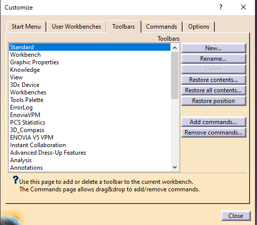
Go to Tools Customize or right click on any toolbar and select Customize to open the dialog box

1-Customizing Toolbars and Start Menu in CATIA V5

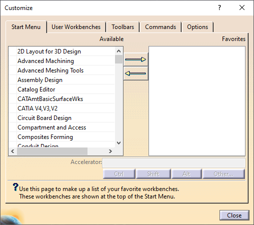
Customize dialog box contains the following tabs:

      • Start Menu: This tool is used to customize the Start Menu where one can add the available workbenches to the list of favourites.
      • User Workbenches: Create your own customized workbench.
      • Toolbars: Shows the toolbars which are visible currently.
      • Commands: These are the commands one can drag and drop to customize the toolbar.
      • Options: Includes general customization options.
      1. Go to Tools Customize Toolbars tab and select New

2-Customizing Toolbars and Start Menu in CATIA V5

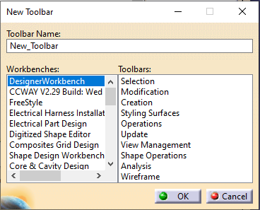
      1. Type the Toolbar Name ➞ Ok.

3-Customizing Toolbars and Start Menu in CATIA V5

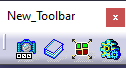
      1. Go to Commands All Commands. Drag and drop the required commands to the New Toolbar as displayed below.

4-Customizing Toolbars and Start Menu in CATIA V5

    1. Customization of existing Toolbars:

One can drag and drop the command onto a toolbar to add it to the toolbar, and drag away the command from the toolbar to delete it.

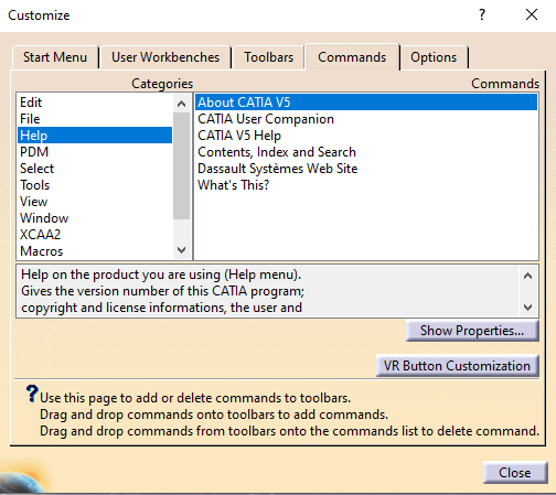
      1. Go to Commands tab which shows the available commands.
      2. One can filter the commands by category, which is listed in the Menu bar.

By selecting Help category, the commands available under it are visible in the Commands area which is displayed below.

5-Customizing Toolbars and Start Menu in CATIA V5

All Commands category shows all commands which are available to use.

If there is any Macro created, it shows the names too. These Macros can then be added to the toolbar.

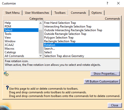
      • Select the required Category and then Command from Commands area.

The Rotation command is selected as displayed in the picture below. Note the icon of the command and a short help message which explains the role of the icon.

6-Customizing Toolbars and Start Menu in CATIA V5

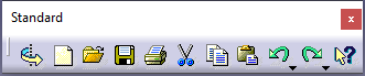
      • To add Rotation command to the Standard toolbar, just drag the command from the above window and drop it on the Standard toolbar as shown below.

7-Customizing Toolbars and Start Menu in CATIA V5

      • To delete Rotation command from the toolbar, drag it away from the toolbar and drop it back to commands list in Customize window.

The commands which don’t have icons can also be dragged and dropped on to the toolbar where their name will be visible as shown below.

8-Customizing Toolbars and Start Menu in CATIA V5

Note:

    • It is not possible to customize the View
    • It is not possible to drag and drop local commands to global toolbars (for example, it is not possible to drag and drop the Pad command to the Standardtoolbar). If one tries, the symbol appears which indicates that this drag and drop is forbidden.
    1. Customizing Start Menu:

Start Menu can be customized by adding the required workbenches to the favourites list.

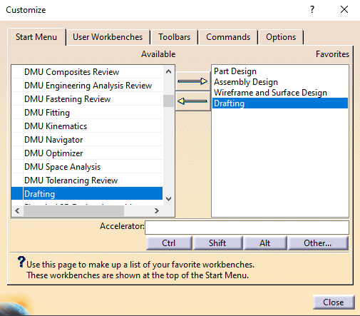
      1. Go to Tools Customize ➞ Start Menu tab
      2. From the available workbenches list, add the required workbenches to the favourites list

9-Customizing Toolbars and Start Menu in CATIA V5

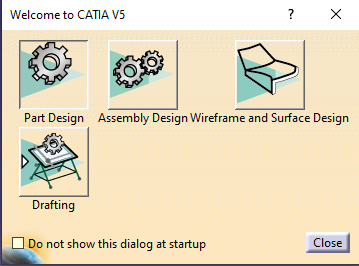
      1. The Start Menu will appear as shown below.

10-Customizing Toolbars and Start Menu in CATIA V5

Environment Variables in CATIA V5

Environment variables in CATIA are used to customize the CATIA environment as per the user requirements.

There are some Environment Variables which help to start CATIA faster. Though they are not documented, they are used by the user community as they work well with the current supported CATIA release.

To add these variables to your current Windows profile:

  • Right click “My Computer”
  • Click “Properties”
  • Click on the “Advanced” tab
  • Click the “Environment Variables” button which will open a new dialog box
  • Under “User variables”, click on “New”
  • Enter the variable name and values from the list below

These Environment Variables can also be added directly to CATIA environment file at location: C:\ProgramData\DassaultSystemes\CATEnv\CATIA.V5-6R20xx.Byy.

Then save the file and restart CATIA.

The most commonly used variables are:

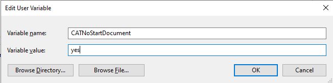
    1. To disable a CAT Product opening on start-up:

CATNoStartDocument = YES

e1

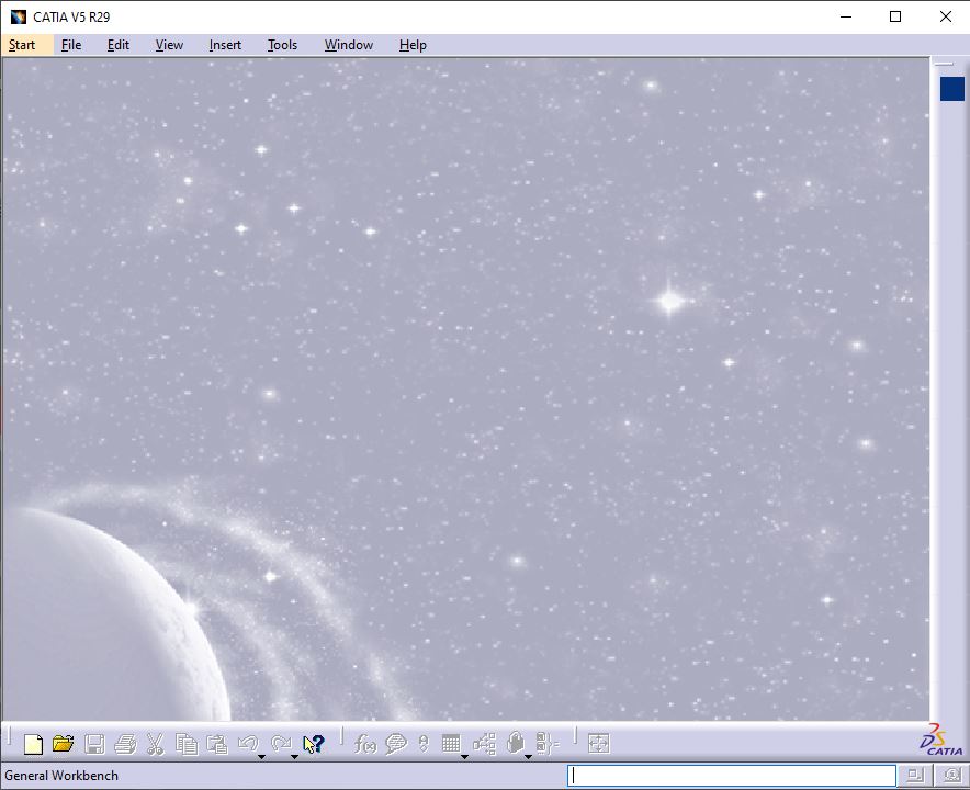
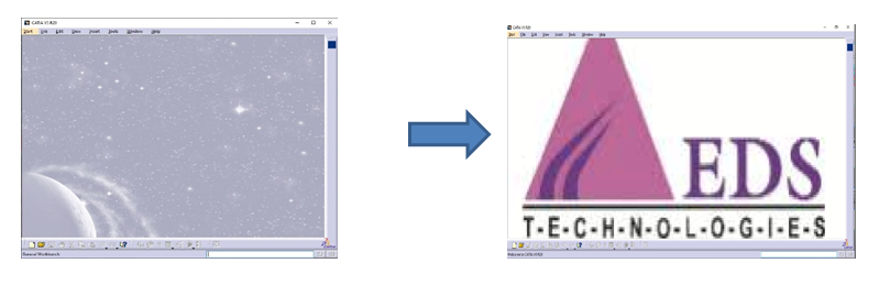
CATIA Startup Screen after using the above Environment Variable:

e2

    1. To disable the galaxy background at start-up:

CNEXTBACKGROUND = NO

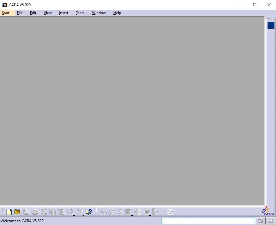
CATIA Startup Screen after using this Environment Variable:

e3

    1. To disable the CATIA splash screen on load:

CNEXTSPLASHSCREEN = NO

If the above Environment Variable is set, CATIA starts without loading the below splash screen.

e4

    1. If you would like to create a custom or company-specific splash screen, all you have to do is replace the file:

C:\ProgramFiles\DassaultSystemes\Bxx\win_b64\resources\graphic\splashscreens\CATIASplash.bmp

Replace the above file with the new file where xx is the version of CATIA you have installed.

e5

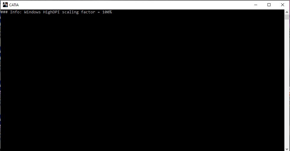
    1. CATIA runs console window/Display CATIA’s logs in command window:

CNEXTOUTPUT = console
e6

    1. The default galaxy background image can also be changed by replacing the file
      C:\ProgramFiles\DassaultSystemes\Bxx\win_b64\resources\graphic\icons\ClientMDIBackgroundNT.bmp where xx is the version of CATIA you have installed.

e7

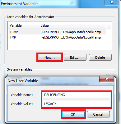
    1. LUM is not supported as a licensing mechanism starting from CATIA V5-6 R2013. In order to use LUM licensing mechanism with CATIA V5 R21 & R22, Environment Variable DSLICENSING with variable value LEGACY should be used by going to Advance System Settings.

e8

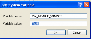
Also, when using CATIA on Windows XP operating system, to communicate with either DSLS or LUM license server, add the following Environment Variable.

e9

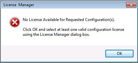
    1. By using following Environment Variable, we can disable license error messages at start-up.

CATLM_ODTS=1

e10

Common Errors and Warnings in Contact and Convergence

While running the analysis on a model with contacts, a major problem arises i.e. convergence. It is not just because of single reason, that it can be resolved in an easy way.  When you come across such problems in different types of analysis, job will terminate by showing an error message or a set of warnings in the analysis. That means the solution is unable to converge.

There are different reasons for why an ABAQUS analysis fails in obtaining the convergence.  The main key area we need to look at is errors and warnings. Almost all symptoms of convergence issue are mentioned in the message file.  The following are some common set of error and warning messages that arise during the convergence:

    1. ERROR: TOO MANY INCREMENTS NEEDED TO COMPLETE THE STEP

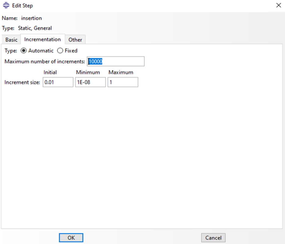
This error arises mainly because of zero pivot or numerical singularity warnings. Check the message file for any warning message. Check the loads and make sure the model can withstand that amount of load and also increase the limit of maximum number of increments in the step.

b1

    1. WARNING: ELEMENT 441 IS DISTORTING SO MUCH THAT IT TURNS INSIDE OUT

This warning is because of Mesh Convergence and it can be fixed by two methods:

    • Refining the mesh into small element length to improve the convergence.
    • By using the complex element type, such as using hybrid formulation, using hourglass enhance technique, etc.
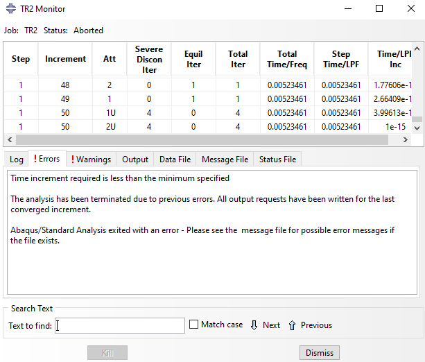
    1. ERROR: TIME INCREMENT REQUIRED IS LESS THAN MINIMUM SPECIFIED -ANALYSIS ENDS

Analysis terminates because the minimum time increment specified is less to achieve the convergence. In the first step, you need to check the message file to see the warnings and error message. To resolve this error, minimum allowable increment size in the step needs to be reduced to obtain the converged solution.

b2

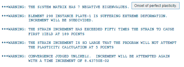
    1. WARNING: THE STRAIN INCREMENT HAS EXCEEDED FIFTY TIMES THE STRAIN TO CAUSE FIRST YIELD AT 500 POINTS

It indicates that the analysis is undergoing excessive plastic yielding which leads to solution inaccuracy and convergence problem. This warning is because of unstable material behaviour. The main cause for this warning is insufficient material data with respect to stress-strain data. The other factors that influence strain increment are: insufficient mesh refinement and unstable deformation, such as buckling. It is always better to extrapolate the plasticity data so that the slope is positive over the range of strain.

b3

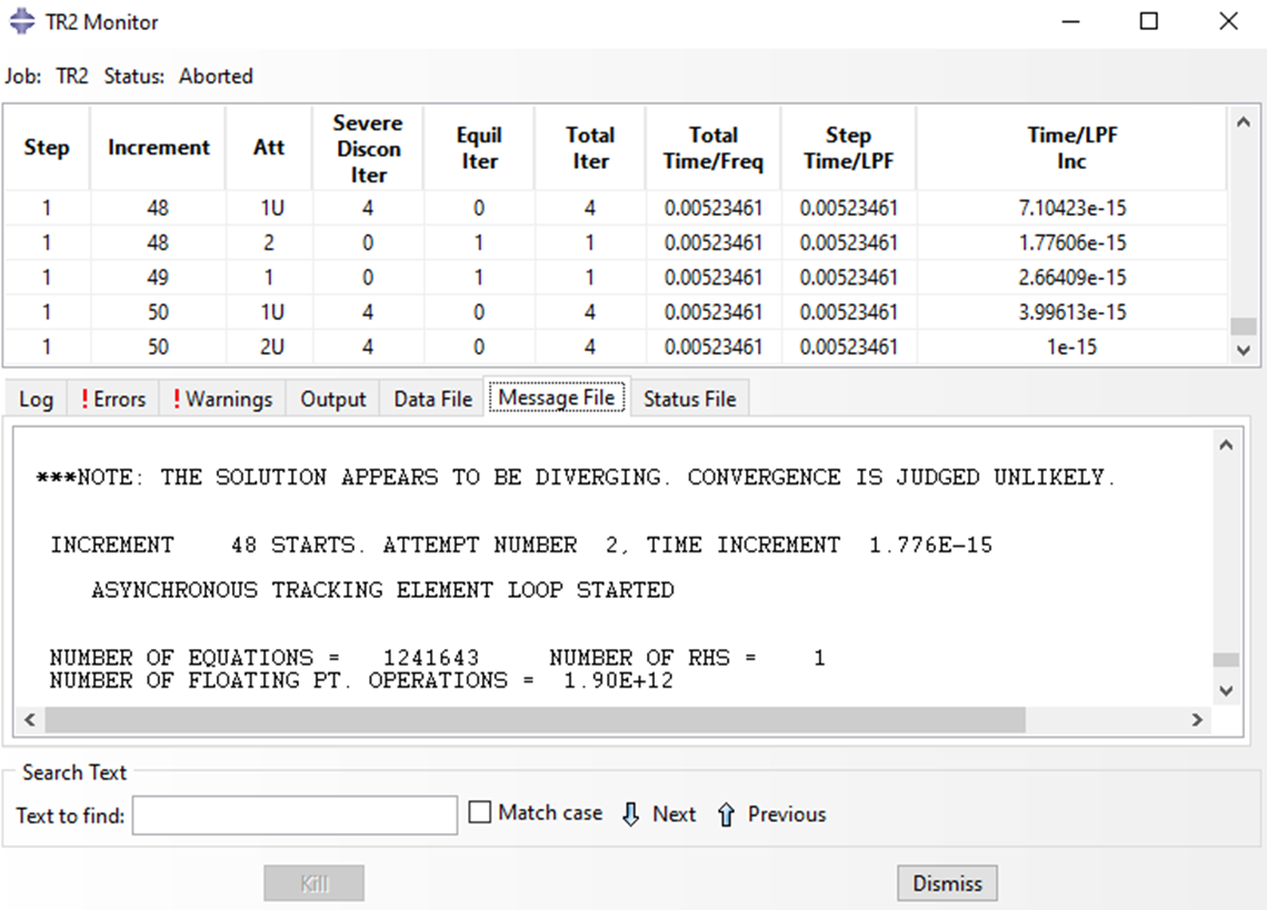
    1. WARNING: THE SOLUTION APPEARS TO BE DIVERGING

This warning message is because of a large increment in the step. Automatic time increment resolves this issue by reducing time increment. It is not a cause for convergence problem but such warnings may lead to cutbacks in analysis.

b4

The majority of convergence problems can be resolved with different approaches. Some of the tips needed to be considered while resolving the convergence problems are mentioned below:

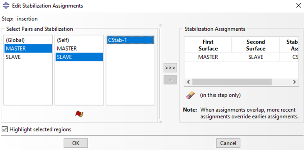
      • Instabilities with respect to contact discontinuity in the analysis directly affect the convergence rate. To overcome local instability due to contact separation, we need to assign the surface wise stabilization in the interaction module by creating the stabilization in contact.

b5

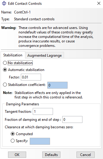
      • Contact non-convergence problem relies on the stability of contact. Keeping that in mind, ABAQUS offers contact controls for stabilization in static problems. Apply the contact controls in order to resolve instabilities in the model during analysis.

b6

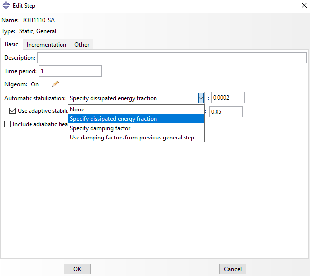
      • Pay attention to warning messages as some of them are specific. If the warning message repeats itself and repeated cutbacks occur, it may indicate a stability issue. This is the most common cause of non-convergence. This can be overcome by specifying the dissipated energy fraction under automatic stabilization in step module.

b7

      • One cause for convergence issue is boundary conditions. If the model is assigned with inadequate boundary condition, it can lead to over or under-constrained conditions. Due to unreasonable boundary conditions, warnings will be generated under job monitor.

The major issue while running contact based problems is convergence and analysis will terminate because of different reasons related to convergence issues. To overcome these problems and to get an accurate output, we need to look at warnings and errors in the message file to judge the aspects responsible for convergence issue in a finite element analysis. Convergence plays an important role in terms of accuracy of simulation problems. So we need to resolve the warnings and errors efficiently to get the required output. I hope this blog has given you the overall solution for convergence problem, considering the most common warnings and error messages.

Understanding DELMIA Virtual Simulation

Typically, in a manufacturing organization, after the design stage and before manufacturing, there is a stage involving planning/PPC and manufacturing engineering. DELMIA (Digital Enterprise Lean Manufacturing Interactive Application) helps organizations to do feasibility study and process validations during detailed process planning immediately after the design stage.

Below are three DELMIA digital manufacturing solutions which can be used in the day-to-day workings of a Simulation Engineer to plan and manufacture.

  • Assembly Simulation
  • While planning for assembly processes, one always needs to take care of feasibility for fitting and disassembly sequence for maintenance purposes. Many organizations perform study on the actual part or the prototype which is expensive and time-consuming. Also, multiple iterations are involved in the study as it is in later stages of design.

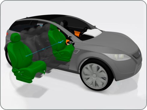
    To avoid these challenges, planners can use virtual tools like Assembly Simulation and simulate the assembly and disassembly sequences and check for multiple possibilities. By doing this, they can validate the assemblies for static and dynamic clash, ease of doing maintenance, tool accessibility etc.

    d1

  • Robotics
  • Many organizations use robots for speed, repeatability and accuracy of work or in hazardous environments like welding. Robot programming with technical support for a particular task is a tedious job and it takes the production time of the robot which is expensive due to loss of productivity.

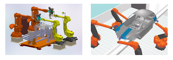
    With DELMIA Robotics, one can teach the robot in the virtual world for welding, material handling, painting, machining, shot peening etc. After validating the program, one can transfer it to the actual robot. After some minor corrections, the robot will work as needed. Hence, the organization can save time and money by using these robots as they can work uninterrupted for a long time.

    d2

  • Ergonomics
  • There are two aspects in ergonomics:

    1. Ergonomics of the shop floor for comfort and safety of the worker.
    2. Product ergonomics for consumer experience.

    At times organizations do ergonomics study by producing expensive prototypes or apply their learnings from previous experiences. Many times one can observe that workers are not productive because of the work environment. Due to this, there is a productivity loss to the company.

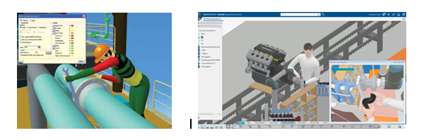
    Using virtual validation of ergonomics, one can improve the work experience of the worker as well as enhance consumer experience. Ergonomics study is useful to ensure comfort, ease of use, reduce fatigue and ensure more productivity. By checking the feasibility and reachability, one can ensure safety and reduction in stress level of the user.

    DELMIA’s ergonomics solutions can help you to do interior design of automobiles and airplanes, work safety analysis and maintenance tasks.

    d3

Performance settings in CATIA V5

There are many ways to manage the performance of CATIA V5 & accuracy of models. To improve performance & increase productivity, we need to configure the settings properly. Some of these options are discussed in detail in this document. These will immensely benefit CATIA users.
    1. Undo Stack

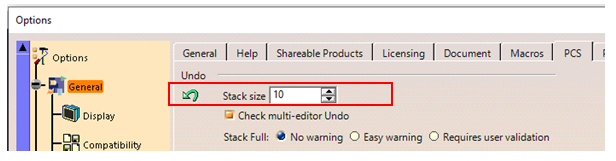
Undo ➞ Stack size ➞ change from 10 to 5

Stack Size defines the maximum number of commands which can be undone for each document. Lower the value better the performance. More the stack value, more will be the memory consumption.

Tools ➞ Options ➞ General ➞ PCS ➞ Undo stack size

a1

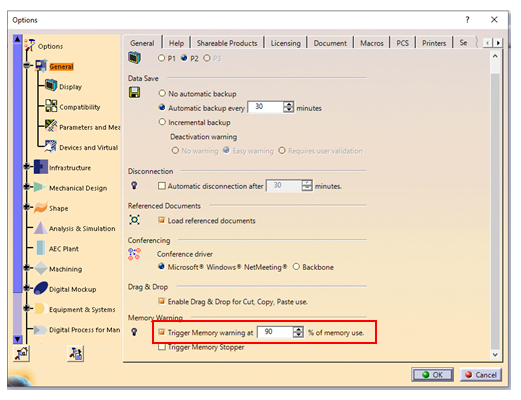
    1. Virtual Memory Setting

Virtual memory of the system should be set to recommended value.

Set trigger memory from 70% to 90%.

A warning message gets activated when the application detects that the memory consumption exceeds the given threshold.

a2

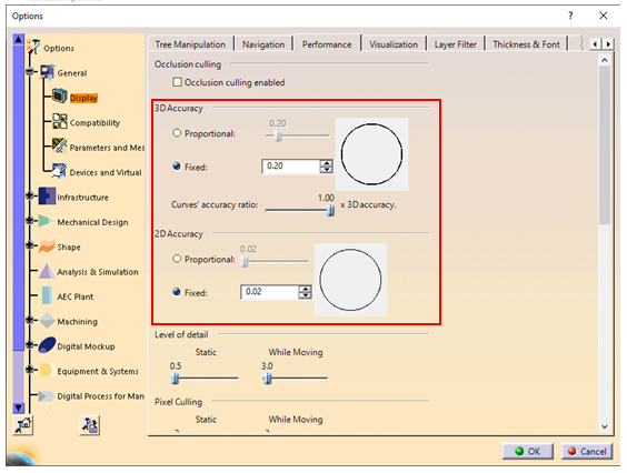
    1. Set 2D and 3D Accuracy for Display

2D and 3D Accuracy settings can be controlled at:

Tools ➞ Options ➞ Display ➞ Performance

Set 2D and 3D Accuracy to maximum value (0.5 or 1.0).

a3

    1. 3D Accuracy Settings for Display

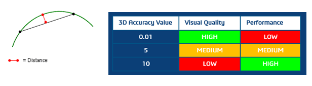
The 3D Accuracy Setting controls the tessellation of surfaces.
Proportional:

Calculating tessellation according to object size. The larger the object, the coarser will be the tessellation. For the same accuracy value, the tessellation on small objects will always be finer than on the larger objects.
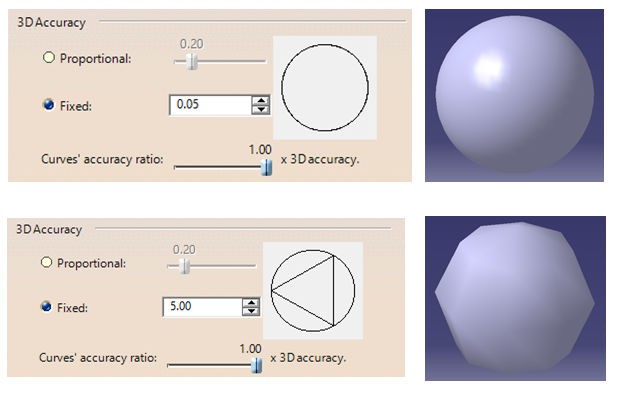
Fixed:

It sets a fixed accuracy value for calculating tessellation on all objects which does not vary with object size.

Capture1 Capture2

In Fixed settings option, user can set a sag value (from 0.01 to 10) for calculating tessellation on all objects which does not vary with object size. The sag value defines the chordal deviation for curves and surfaces.

    1. Pixel Culling
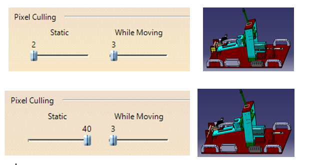
      • The minimum object size in pixels technology is used to define the size in pixels of objects to be displayed or hidden in the geometry.
      • Setting a high value enables to quickly move large parts.
      • Setting a low value displays more details. For example, setting a value of 2 means that objects whose size on screen is lower than 2 pixels are static.

a7

    1. Anti-Aliasing
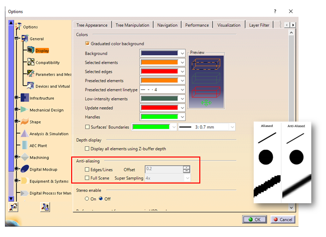
      • This technology is used to smooth out the uneven edges of objects.
      • For better performance, anti-aliasing should be disabled.

Tools ➞ Options ➞ General ➞ Display ➞ Visualization

a9

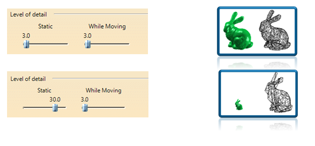
    1. Level of Detail (LOD)
      • The Level of Detail technology or LOD adjusts the polygonal representation of an object to the distance of the user. The idea is that it is not always necessary to view a high level of detail in the geometry because some objects are far away, enough to make the detail meaningless.
      • Set a high value to remove details.
      • Set a low value to see all details.

a10

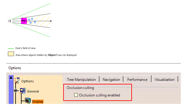
    1. Occlusion Culling
      • The occlusion culling technology improves rendering performance by rendering visible objects only. It is used to detect and prevent occluded objects from being rendered.
      • Occlusion culling optimizes memory consumption and CPU usage.
      • Recommended for large and highly compartmented assemblies.

a11

      • Use approximate mode for creating views in drafting.

Tools ➞ options ➞ Mechanical design ➞  drafting ➞ View ➞ View generation mode ➞  approximate view

      • Use CGR management while working on large assemblies.

Tools ➞ options ➞  Infrastructure  ➞ Product Infrastructure  ➞ Cache management ➞ Check work with cache system

      • Proper CATIA Media Setup

CATIA V5 64 bit is to be installed on a 64-bit machine. Also install updated service packs for respective release on GA code.

      • Recommended DS Hardware

System configuration should be as recommended by Dassault Systèmes. Refer the below link.

https://www.3ds.com/support/hardware-and-software/

      • Cleaning Data

Assembly cleaning: Regularly clean the assembly as mentioned below:

Files  ➞ desk  ➞ right click on part/product  ➞  CATDUAV5 ➞  select priority 3 ➞ check clean option at bottom  ➞ RUN

Repeat this procedure for all parts and products.

      • Corrupted CATSettings

Delete corrupted CATSetting.

For Operating System: Windows XP

C:\Documents and Settings\Administrator (User Name) \Application Data\DassaultSystemes\CATSettings

For Operating System: Winows7/10

C\User\Username\App Data\ DassaultSystemes\Roaming\CATSettings

Delete all files in CATSettings folder (except licensing file).

Subscribe to our newsletter

Get all the latest information on Events, Sales and Offers.